Augmented Shanahan: Detection
 Click here to view.
When I was thinking of ideas for the 5C Hackathon back in November, I thought it would be really cool to do augmented reality on buildings. They are large, somewhat unnoticed features of the environment, and they are relatively static, not moving or changing over time. They seemed like the perfect thing to overlay with augmented reality. And since they are so large, it opens up the possibility for multiple people to interact with the same wall simultaneously.
Note: This is mostly an explanation of how I implemented detection. If you prefer, you can skip ahead to the 3D extrapolation and rendering in part 2, or to the game logic in part 3.
If you instead want to try it out on your own, click here. The augmented reality works on non-iOS devices with a back-facing camera and a modern browser, but you have to be in the Shanahan building to get the full effect. Denying camera access or accessing it on an incompatible device will use a static image of the building instead of using the device camera. Works best in evenly-lit conditions. Image quality and detection may be slightly better in Firefox than Chrome, which doesn't autofocus very well.
After completing the augmented reality snake game at the hackathon, I started thinking of ways to do a similar thing with a particular wall on a specific building, the Shanahan Center for Teaching and Learning:

Originally, I chose this wall for a few reasons. First of all, it was far away from obstructions. The Shanahan building has an opening in the middle, so you can look at this wall from the opposite side of the second floor, without having to worry about people walking in front. Secondly, it has some distinctive features, such as the four windows, that make it pretty ideal for a game.
I considered a few ways to recognize this wall. My first attempt was to use ORB (Oriented and Rotated BRIEF) feature descriptors and the YAPE feature detector that are provided with the JSFeat library. Basically, the YAPE feature detector scans the image for high-contrast, distinctive points that would likely be similar from different viewpoints. Then, for each point, an ORB descriptor is calculated by comparing the relative intensities of pixel pairs around that point. The pixel pairs are randomly distributed, but are only generated once and thus have the same offsets from each point.
Depending on which pixel in the pair is brighter, the pair is tagged either 0 or 1. Then, all of the tags are concatenated together to form a vector of zeroes and ones, which is converted into a number. That number is the ORB descriptor for that point.
To match an object in an image, a program can run the algorithm on that image, and then compare each point's descriptor with all the descriptors of the original image of the object to find which points in the new image correspond to which other points in the old image. Then those correspondances can be used to estimate the position of the object in the new image (in this case as a perspective transformation matrix).
Unfortunately, this didn't work very well in this particular case. It could only detect the wall in very specific lighting conditions and orientations. My guess is that it failed for a few reasons:
- The YAPE feature detector was not consistent in the points it picked. Feature detectors like YAPE are designed for highly textured objects, and the lack of many high-contrast features made it so that the YAPE detector tended to pick inconsistent specks in the image.
- The ORB detector is highly sensitive to scale, so dealing with different sizes of the target was difficult.
- The features on the wall are not very distinctive. As it is essentially a grid of squares with four similar-looking windows, it is difficult for the algorithm to accurately match points.
I was thus left with the problem of figuring out another method to detect the wall. Looking at the image, the first thing that came to mind was to detect the windows. Unfortunately, that ended up being harder than it looked.
First of all, the lighting is not consistent across the image, or from image to image. Unless we picked the perfect threshold, that would make it difficult to detect the windows in every frame.
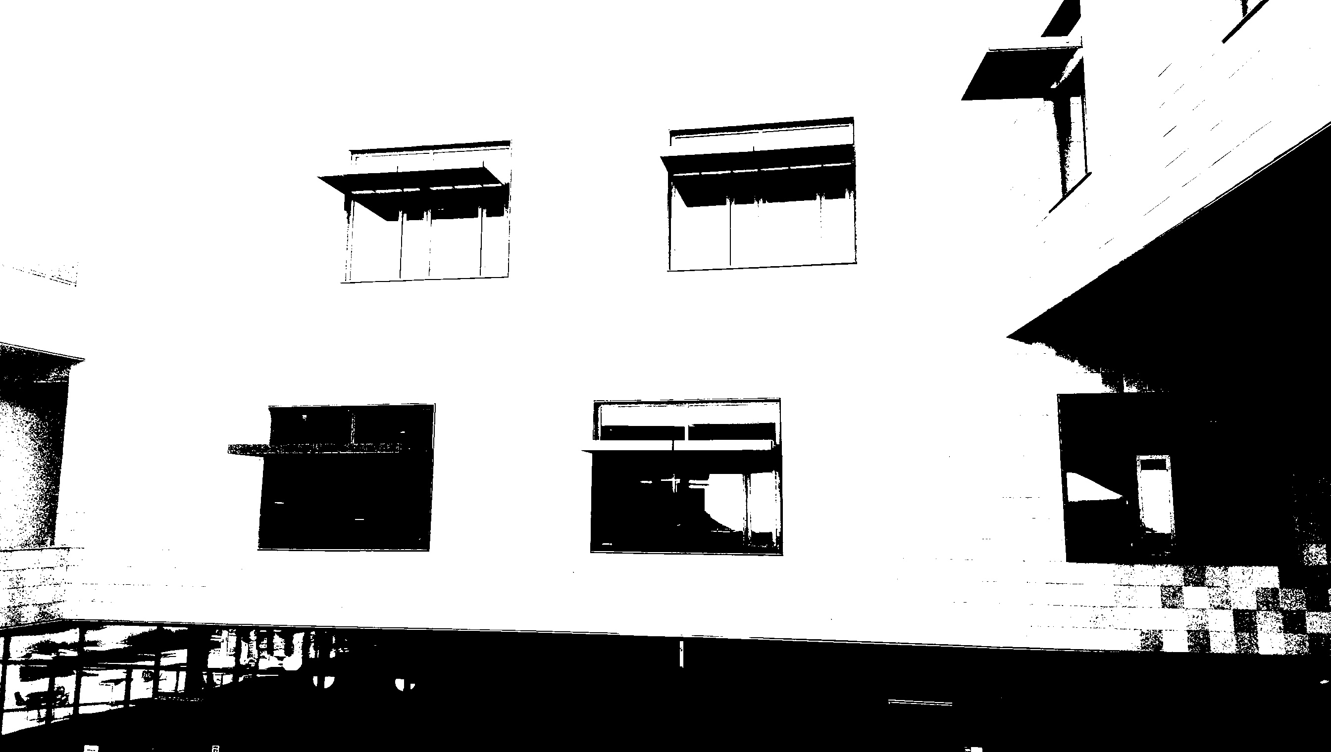
If I attempted to detect the edges of the windows, I ran into similar problems: the edges between differently colored squares were stronger in some cases than between the window edge and the squares.


And even if I could reliably isolate the windows from the background noise, it would be difficult to get useful information from them. The edges of the windows were often fuzzy and incomplete (notice the gaps in the edges of the upper windows in the thresholded image due to the lightness of the window overhang, and the gaps in the edges of the lower windows due to the lower contrast). Furthermore, the window overhangs that protrude from each window make the outlines of the windows non-rectangular, making the identification of the true corners difficult.
While attempting to find a more robust window detection method, however, I stumbled upon something interesting. I had tried to subtract each pixel from the mean of the pixels around it to generate a more relative threshhold, and accidentally produced the following image:
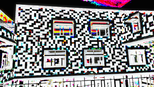
This is actually mostly an artifact of the fact that the image I was working with used unsigned 8-bit integers. Thus when I subtracted two numbers, if the result was negative (i.e. 40 - 45) then since each pixel could only hold values between 0 and 255, it overflowed to a very high value (i.e. 40 - 45 = 250) and appeared almost white, whereas if the result was positive, it was generally very small and thus appeared black. But it got me thinking about the pattern of lightness and darkness in the squares of the building.
I realized that, since there are many different colors of square, arranged randomly, each region of the wall has a slightly different pattern. If we took a specific group of nine adjacent squares, we could probably identify the location of that group on the wall based only on the colors of the squares.
The algorithm I ended up using to detect the wall was based on this idea, combined with the concepts from the ORB feature detector. Instead of attempting to find points of high contrast, however, I instead wanted to find squares. Then I could use the pattern of light and dark around that square to generate my own descriptor and match its with a precomputed set of descriptors for each square on the wall.
To detect squares, I employed a relatively simple algorithm:
- Pick a random point in the image.
- Walk in all four directions (up, down, left, right) until hitting a pixel that is significantly different in intensity (I experimentally found 15 to be a good threshold for differentness).
- Assuming that this point is in a square, then the center of the square can be found by taking the midpoint between the left and right spans and the upper and lower spans (i.e. if we went 3 pixels left and 17 pixels right before stopping at an intensity change, then the center of the square is likely at around 7 pixels to the right of the random point, which would put it equally between the two stopping pixels).
- Walk in all four directions from this new point until hitting a pixel that is significantly different in intensity.
- Check if all four directions went a similar number of pixels. If so, we have likely identified a square, and the size of the square is the average of its width and height. If not, throw this point away and pick another random point.
- Repeat until we have enough points.
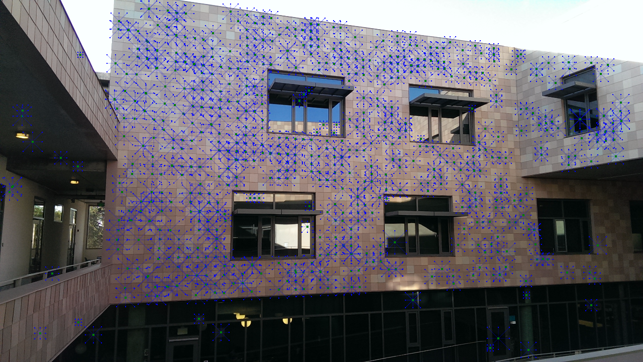
In this image, we can see the process of finding the points. The blue lines are the initial four directions walked, starting with a random point, and then the red and green lines show the estimated center and the updated walks. Green lines are close enough in length to be considered squares, and red lines are too different and are thus discarded.
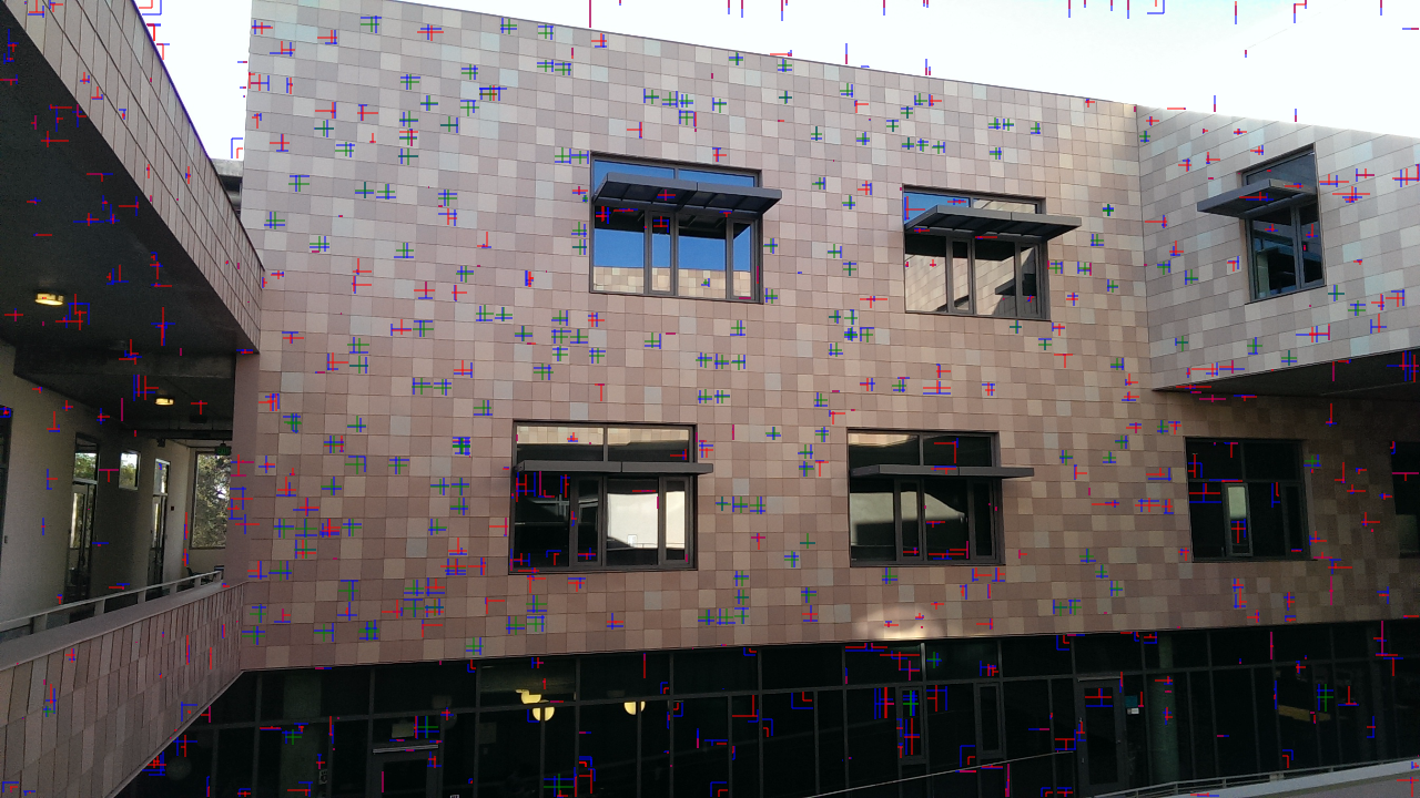
We can then use the calculated size of the square to find the centers of the squares adjacent to it (assuming there are squares there), which are colored blue in this image. Note that this image used a very large number of sample points, and does not show any of the test points that were determined not to be squares.
For each of these found squares, we can find the intensities of all of the neighboring squares, and then use those intensities to create a descriptor vector. For example, comparing the first two squares, if the first one is greater than the second, we assign the pair 10 (2 in binary) and if the second one is greater than the first, we assign the pair 01 (1 in binary). If both seem about equal in intensity, we give the pair a 00 (0 in binary). This is repeated for all pairs of squares in the nine-square neighborhood for a total of 36 pairs, or 72 binary digits. This bit string is our descriptor.
We can then compare these descriptors with a database of all known descriptors (calculated in advance). To compare two descriptors, we count how many of the binary digits do not match. This is known as the Hamming distance between the two descriptor vectors. For example, the bit strings 10010101 and 00110101 have a Hamming distance of 2. We keep track of the best match, and if the best match has a small enough distance (7 or fewer wrong digits out of 72 seemed to work well) we mark it as a good match.
We now have a set of many potential matches, some of which may be incorrect, and we want a perspective transformation matrix that maps the first set of points to the second set. It turns out that there is a method designed to do exactly that, known as RANSAC. The basic idea of RANSAC is to pick a few random points, fit a model to them, and then see how many other points agree with that model. The number of points that agree is then the score of that model, and if this is greater than the number of points that agreed with the last model, we throw away the old model in favor of this one. If we do this enough times, and enough of our points are not outliers, the points that agreed with the best model are probably all inliers, and we can either use that model or attempt to make a more accurate model by simply fitting the model to the likely inliers.
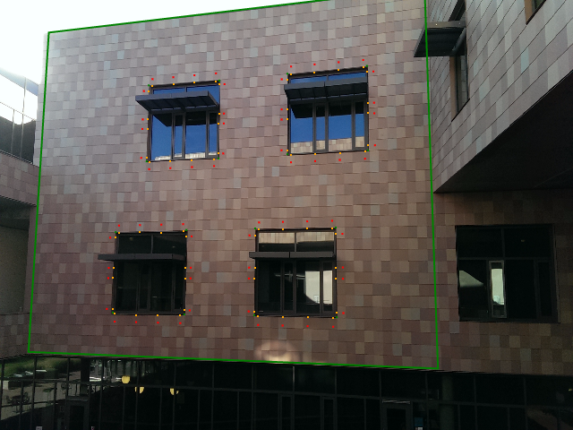
Using the JSFeat library, it is easy to do RANSAC with a perspective transform homography. The resulting transformation matrix for this viewpont can be seen below. Note that the orange lines are drawn from the randomly chosen square to the position of that square predicted by the best-fit transformation matrix. For the correctly-identified squares, the orange line is more of an orange dot, as they are only off by a few pixels. For the few outliers, however, the line points at a different square: this is the square that best matched the pattern of intensities. Predictably, with most of the false matches, the incorrect location has a very similar pattern as the correct location.

Ultimately, as I was experimenting with different lighting conditions, I had to modify threshholds in favor of bad matches. I originally allowed only very good matches (distance 4 or less) to participate in the model fitting, but in different lighting conditions that resulted in a very small number of good matches, preventing me from finding a good matching. I ended up allowing even relatively tentative matches to be marked as good because the RANSAC algorithm proved to be quite effective at removing outliers even if there were many of them.
At this point, I had successfully detected the wall in a single frame. This method, however, is not consistent enough to use alone. Although it can detect the wall in specific lighting conditions very reliably, in other lighting conditions it takes a few frames before a correct match is found. Thus if I tried to use just this method, the match would flicker in and out. Once I have a successful match, however, tracking it is an easier problem.
To track the wall after it is found, I used the Lucas-Kanade optical flow method. This method tracks points by assuming that, around a specific point, the displacements are a small translation (linear motion, no rotation or scaling). Thus the change in the intensity of each pixel is approximately the sum of the intensity derivative with respect to x times the x velocity and the intensity derivative with respect to y times the y velocity. In math notation, for a given pixel $q_n$,
$$I_x(q_n) \times V_x + I_y(q_n) \times V_y = -I_t(q_n)$$
where $V_x$ and $V_y$ are the displacements of the point and $I_x$, $I_y$, and $I_t$ are the x, y, and time derivatives of the intensity at a given point.
Conveniently, Lucas-Kanade flow tracking is provided by the JSFeat library, so I simply asked the library to track the four corner points of each window. Since some of the corners might be covered by other objects in the view and thus track the wrong motion, I then used RANSAC on the resulting tracked points to identify any incorrectly tracked points and calculate an updated transformation.
In addition, I wanted to make sure that the initial transformation as well as the tracked and updated transformations were accurate. To do this, I check to make sure that the windows were where they should be. I choose a set of test points in the squares around the window and, for each point, walk inward toward the window until hitting a pixel that was significantly darker than the start pixel. I then use the found points to estimate the window edge lines, and then intersect the lines to find where the window corners should be. If too few of the corners are found in a given frame, I discard the transformation. Otherwise, I use the found corner points and RANSAC to refine my estimate of the transformation.
To prevent jitter when the camera image is steady, if the transformation was valid in the last frame and the Lucas-Kanade flow tracking shows very small movement, I skip refining the transformation based on the window detection, instead simply using the Lucas-Kanade transformation. Only when the points move a large amount do I use the window tracking to refine the initial estimate.
By combining a custom, square-based feature detector and descriptor with RANSAC, Lucas-Kanade feature tracking, and window corner checking, I was able to accurately and reliably locate the wall and track it between frames. The next step was to use the calculated transformation to render in 3D on top of the wall. I will discuss how I accomplished that in part 2 of this writeup.